
Are you considering letting or selling a property, or renting or buying? I am a management consultant specialising in business valuation and would like to explain the valuation of real estate to you. Estimating future investments may be the job of a civil engineer, but the mathematics of valuing companies and real estate are identical.
Unfortunately, I see time and again that wrong decisions are made when buying and selling real estate. These are decisions with considerable consequences. The following explanations are intended to help prevent wrong decisions. The aim is for you to understand how the value of a real estate property is determined.
Once you have understood what actually happens when calculating the value of real estate, you will find a guide to calculating it yourself using the capitalised earnings method (original) below.
It is important that a distinction is made between value and price in a real estate valuation. Unfortunately, these two words are often confused. The decision value is subjective (dependent on the individual) and takes into account the individual decision field (e.g. taxes, losses carried forward, alternative investments, withdrawal preferences, etc.) and is the most important value that characterises the limit of advantageousness.
The benefit of the future cash flow is discounted to the present using a calculation interest rate (endogenous marginal interest rate).
In addition to the decision value, there is an arbitration value (arbitrator value), which an independent expert can calculate from the decision values of the parties involved. Argumentation values are values for influencing negotiations, which can be based on more or less plausible procedures.
Two further values should be mentioned. The liquidation value (sale of all assets) is regarded as the lower value limit in business valuation. The reconstruction value is more important in the context of real estate valuation and corresponds to the new construction of the real estate including the acquisition of the land. In the business valuation, it corresponds to a new foundation.
The price, on the other hand, is the amount paid in a transaction. It regularly deviates from the decision value.
The familiar capitalised earnings method in accordance with the ImmoWertV does not actually calculate values, but rather market prices based on market data. The transformation factor is the property interest rate. Roughly speaking, this works as follows:
However, the property interest rate is a kind of “black box” that implies a lot of data and should not be used for investment decisions. Why? It implies the overall development of relevant factors (yield curve, inflation, population, economy, etc.).
In a property bubble, the property interest rate tends to fall further and further. A low interest rate causes property prices and values to rise massively. As the property interest rate is derived from market data, the capitalised earnings method in accordance with ImmoWertV justifies inappropriately high prices in property bubbles. The situation is different with the functional valuation theory and the closely related original capitalised earnings method (Hering, 2017; Hering 2021; Matschke & Brösel, 2013; Toll, 2011, Walochnik, 2021).
Explanations of the capitalised earnings method in various forms, including according to the ImmoWertV, can be found on the linked page on the capitalised earnings method. The capitalised earnings method in accordance with ImmoWertV is justified within the legal scope of application.
Below you can see a graph that shows how strongly the interest rate influences the real estate value. If a perpetual annuity is discounted at an interest rate of 10%, the value is 120000 monetary units (MU). At an interest rate of 5% it is already 240000 MU and at an interest rate of 1% it is 1200000 MU.
Figure 1: Discounting of a Perpetual Annuity
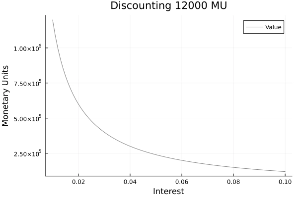
Source: own presentation.
This section looks at the question of when it is worth letting and when it is worth selling real estate. The examples are abstracted from real-life circumstances so that they are easy to understand. Complex calculations (progressive taxes, losses carried forward, etc.) are not taken into account in the explanations here.
Mr Immanuel Biele lives alone and has an annual gross salary of 50,000 monetary units (MU) and rents out a property for 12000 MU per year. Both are taxed at a rate of 30%. The necessary living expenses amount to 10000 MU. Investments at the bank can be made at 5%. Investments are taxed at 25%, so the net interest rate is 0.05*(1-0.25) = 3.75%. (Formulas for net interest rates can be found in Schneeloch et al. (2020)).
In the base case there is no inflation, in the modification there is growth (inflation) of 2%. Salary, cost of living and rent develop in line with inflation (indexation).
Immanuel Biele is faced with the question of whether he should continue to rent out his real estate or rather sell it. He looks for his decision value. This is the value at which the advantageousness changes.
In the case of renting without inflation, Immanuel Biele has a salary of 50000 MU and rental income of 12000 MU. Living expenses are available in the amount of 10000 MU. After taxation and deduction of essential living expenses, he has (50000+12000)*(1-0.3)- 10000= 33400 MU per year at his free disposal (withdrawal). He uses this in particular for leisure activities and holidays.
Table 1: Letting Real Estate without Growth
| Description | Year 1 | Year 2 | Year 3 | Year ... |
|---|---|---|---|---|
| Salary | 50000 | 50000 | 50000 | ... |
| Rental Income | 12000 | 12000 | 12000 | ... |
| Tax | -18600 | -18600 | -18600 | ... |
| Cost of Living | -10000 | -10000 | -10000 | ... |
| Withdrawal | -33400 | -33400 | -33400 | ... |
Source: own presentation.
The case is similar to the above case with the addition that his salary, rental income and cost of living are adjusted for inflation.
| Description | Year 1 | Year 2 | Year 3 | Year ... |
|---|---|---|---|---|
| Salary | 50000 | 51000 | 52020 | ... |
| Rental Income | 12000 | 12240 | 12484.8 | ... |
| Tax | -18600 | -18972 | -19351.44 | ... |
| Cost of Living | -10000 | -10200 | -10404 | ... |
| Withdrawal | -33400 | -34068 | -34749.36 | ... |
Source: own presentation.
Immanuel Biele is considering selling his real estate. An expert for the valuation of real estate and businesses tells him that with a value (decision value) of at least 224000 MU, he can receive the same withdrawal stream as if he were renting. He provides him with the following financial plan for clarification.
The calculation interest rate (endogenous marginal interest rate) is 0.05*(1-0.25)=0.0375. The perpetual annuity is equal to 120000*(1-0.3)/0.0375 = 224000 MU.
(The rent was taxed at 30%, capital gains are only taxed at 25%. The net result of the rental income 12000*(1-0.3) and the interest income (11200*(1-0.25)) is the same amount of 8400 MU.)
Table 3: Real Estate Value Calculation excl. Growth and Taxes
| Description | Year 1 | Year 2 | Year 3 | Year ... |
|---|---|---|---|---|
| Salary | 50000 | 50000 | 50000 | ... |
| Interest Income | 11200 | 11200 | 11200 | ... |
| Tax | -15000 | -15000 | -15000 | ... |
| Tax on Interest | -2800 | -2800 | -2800 | ... |
| Costs of Living | -10000 | -10000 | -10000 | ... |
| Withdrawal | -33400 | -33400 | -33400 | ... |
| Capital | 224000 | 224000 | 224000 | ... |
Source: own presentation.
In the following case, the valuer takes into account inflation and thus the price increase. The decision value, i.e. the value at which the advantageousness of selling or renting is determined, is 480000 MU. In this case too, the valuer draws up a financial plan for the valuation of real estate and businesses.
The calculation interest rate (endogenous marginal interest rate) is 0.05*(1-0.25)=0.0375. As a perpetual annuity with growth, this results equally in 120000*(1-0.3)/(0.0375-0.02) = 480000 MU.
Table 4: Real Estate Value Calculation incl. Growth and Taxes
| Description | Year 1 | Year 2 | Year 3 | Year ... |
|---|---|---|---|---|
| Salary | 50000 | 51000 | 52020 | ... |
| Interest Income | 24000 | 24480 | 24969.6 | ... |
| Tax | -15000 | -15300 | -15606 | ... |
| Tax on Interest | -6000 | -6120 | -6242.4 | ... |
| Cost of Living | -10000 | -10200 | -10404 | ... |
| Withdrawal | -33400 | -34068 | -34749.36 | ... |
| Capital | 480000 | 489600 | 499392 | ... |
Source: own presentation.
The examples show that in a real estate valuation, the withdrawal flow must at least correspond to the initial situation. The minimum amount that must be obtained in order to achieve this withdrawal flow is then sought. In technical terms, this is known as the base program and then the valuation program. Of course, in the real world, much more information must be included in the valuation, such as progressive taxes, losses carried forward, risk, etc.
What is particularly important is what is done with the money after the sale. Is it invested in a bank at a low interest rate? Will the money be invested in shares on the capital market? Will the sale be used to pay off a high-interest loan? The decision value depends on the individual situation (alternative investment). Figure 2 shows the effect of the alternative investment again. The higher the alternative interest rate in the above case, the lower the decision value when selling the real estate. It can also be concluded from this that a sale without alternative use is pointless (interest rate of 0%).
Figure 2: Discounting Investment Alternative Sale
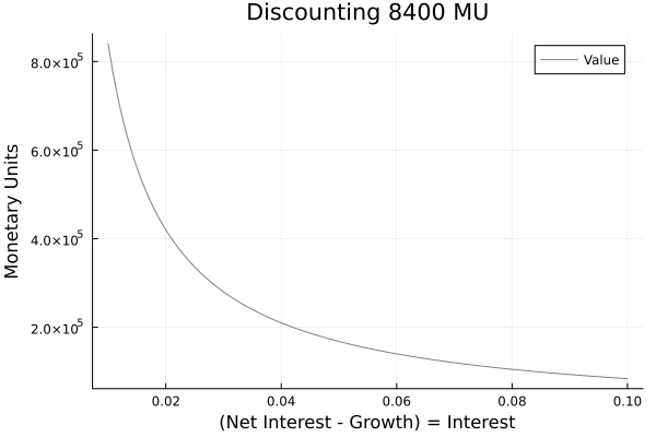
Source: own presentation.
This section looks at the question of when it is worth renting and when it is worth acquiring real estate. The examples are abstracted from real-life circumstances so that they are easy to understand. Complex calculations (progressive taxes, losses carried forward, etc.) are not taken into account in the explanations here.
Mr Immanuel Biele lives alone and has an annual gross salary of 50,000 MU. This is taxed at a rate of 30%. The necessary living expenses amount to 10000 MU. In addition, he can either rent a property for 12000 MU per year or acquire one for a currently unknown price. Specifically, he can either rent one side of a semi-detached house or acquire the other side.
In the base case there is no inflation, in the variation there is growth (inflation) of 2%. Salary, cost of living and rent develop in line with inflation (indexation).
Investments at the bank can be made at 5%. Investments are taxed at 25%, so the net interest rate is 0.05*(1-0.25) = 3.75%. (Formulas for net interest rates can be found in Schneeloch et al. (2020)).
There are further case distinctions for loans.
In the first case group, unlimited loans can be taken out for 10%. In the other case group, an instalment loan (annuity loan) can be taken out over 10 years for 10% and is linked to the acquisition price (mathematically through a restriction in a linear programme). The loan can be represented as a cash flow as follows:
Without inflation: [1, -0.1627, -0.1627, -0.1627, -0.1627, -0.1627, -0.1627, -0.1627, -0.1627, -0.1627, -0.1627, -0.1627]
With inflation: [1, -0.1509, -0.154, -0.157, -0.1602, -0.1634, -0.1666, -0.17, -0.1734, -0.1768, -0.1804]
Immanuel Biele is faced with the question of whether he should rent or acquire real estate. He is looking for his decision value. This is the value at which the advantageousness changes.
In the case of rent without growth (inflation), Immanuel Biele has a salary of 50000 MU. He pays 15000 MU tax on this. The necessary living costs amount to 10000 MU and the rent to 12000 MU per year. He has 50000 – 15000 – 10000 – 12000 = 13000 MU at his disposal (withdrawal). He uses this in particular for leisure activities and holidays.
| Description | Year 1 | Year 2 | Year 3 | Year... |
|---|---|---|---|---|
| Salary | 50000 | 50000 | 50000 | ... |
| Tax | -15000 | -15000 | -15000 | ... |
| Cost of Living | -10000 | -10000 | -10000 | ... |
| Rent | -12000 | -12000 | -12000 | ... |
| Withdrawal | -13000 | -13000 | -13000 | ... |
Source: own presentation.
The case is similar to the above case with the addition that his salary, cost of living and rent are adjusted for inflation.
| Description | Year 1 | Year 2 | Jahr 3 | Year... |
|---|---|---|---|---|
| Salary | 50000 | 51000 | 52020 | ... |
| Tax | -15000 | -15300 | - 15606 | ... |
| Cost of Living | -10000 | -10200 | -10404 | ... |
| Rent | -12000 | -12240 | -12484.8 | ... |
| Withdrawal | -13000 | -13260 | -13525.2 | ... |
Source: own presentation.
In the case of real estate acquisition, two groups of cases will be presented. This is followed by a few variations in tables.
In the first case group (extreme case), only the interest on the loan (no annuity loan) and no amortisation is paid.
In the second case group, an annuity loan is taken out in the amount of the acquisition price. Immanuel Biele avoids further loans.
Please note: The following explanations do not apply to a real estate acquisition for investment purposes, i.e. for letting. In this case, taxes on the rental income in particular must be taken into account.
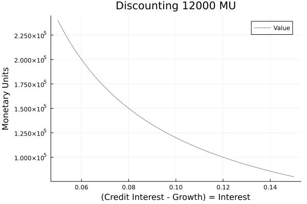
In an extreme case, Immanuel Biele only pays the interest. An expert for the valuation of real estate and businesses tells him that with a value (decision value) of 120000 MU, he can receive the same withdrawal stream as with rent. He provides him with the following financial plan for clarification.It becomes clear that he only pays the interest of 12000 MU without ever repaying.
The calculation interest rate (endogenous marginal interest rate) is 0.1. 120000/0.1 = 120000 MU calculated as a perpetual annuity.
| Description | Year 1 | Year 2 | Year 3 | Year ... |
|---|---|---|---|---|
| Salary | 50000 | 50000 | 50000 | ... |
| Tax | -15000 | -15000 | -15000 | ... |
| Cost of Living | -10000 | -10000 | -10000 | ... |
| Acquisition | -120000 | 0 | 0 | ... |
| Interest | -12000 | -12000 | -12000 | ... |
| Repayment | -0 | -0 | -0 | ... |
| Withdrawal | -13000 | -13000 | -13000 | ... |
| Credit | 120000 | 120000 | 120000 | ... |
Source: own presentation.
In the modification, the valuer takes into account inflation and thus the price increase.The decision value, i.e. the value at which the advantageousness between buying and renting is determined, is 150000 MU. In this case too, the valuer draws up a financial plan for the valuation of real estate and businesses. Only the interest is repaid and the loan increases annually so that the interest can just be serviced. (The purchasing power and the rent saved increase.)
The calculation interest rate (endogenous marginal interest rate) is 0.1. Alternatively, a perpetual annuity with growth can be discounted for the calculation 120000/(0.1-0.02) = 150000 MU.
| Description | Year 1 | Year 2 | Year 3 | Year ... |
|---|---|---|---|---|
| Salary | 50000 | 51000 | 52020 | ... |
| Tax | -15000 | -15300 | - 15606 | ... |
| Cost of Living | -10000 | -10200 | -10404 | ... |
| Acquisition | -150000 | 0 | 0 | ... |
| Interest | -15000 | -15300 | -15606 | ... |
| Repayment | -0 | -0 | -0 | ... |
| Withdrawal | -13000 | -13260 | -13525.2 | ... |
| Credit | 150000 | 153000 | 156060 | ... |
Source: own presentation.
Immanuel Biele takes out a loan from his bank in the amount of the acquisition price. The loan (annuity loan) has an interest rate of 10% and is repaid over 10 years. After that, he wants to remain credit-free.
An expert for the valuation of property and companies tells him that with a maximum value (decision value) of 73734.81 MU, he can obtain the same withdrawal rate as for rent. He provides him with the following financial plan for clarification.
The calculation interest rate (endogenous marginal interest rate) is 0.1.
The value of 73734.81 MU can also be calculated using the formula for the present value factor bwf(i,n) = ((i+1)^n-1)/((1+i)^n*i). The result is 12000 * 6.14 = 73734.81 MU. If Immanuel Biele were to allow unlimited indebtedness, as in the extreme case, he could discount the rental income saved after paying off the loan. The endogenous marginal interest rate is the loan interest rate of 0.1. The value is (12000/0.1) *(1+0.1)^(-10) = 46265.19 MU. Together this results in 46265.19 + 73734.81 = 12000 MU. This is the value from the extreme case.
(For mathematicians: The marginal price was calculated in two ways using a linear programme. Firstly by means of an annuity loan, which was linked to the acquisition price. And once through a restriction in year 10, which prevents debt. In the first case, the dual value of the liquidity restriction in t=1 corresponds to the present value factor of 6.14. In the second case, the endogenous marginal interest rate of 0.1 can be calculated using the dual values of the liquidity restriction.)
Tabelle 9: Acquisition of Real Estate without Growth (10-Year Annuity Loan)
| Description | Year 1 | Year 2 | Year 3 | Year ... |
|---|---|---|---|---|
| Salary | 50000 | 50000 | 50000 | ... |
| Tax | -15000 | -15000 | -15000 | ... |
| Cost of Living | -10000 | -10000 | -10000 | ... |
| Acquisition | -73734.81 | 0 | 0 | ... |
| Interest | -7373.48 | -6910.83 | -6401.91 | ... |
| Repayment | -4626.52 | -5089.17 | -5598.09 | ... |
| Withdrawal | -13000 | -13000 | -13000 | ... |
| Credit | 73734.81 | 69108.29 | 64019.11 | ... |
Source: own presentation.
In the following case (annuity loan), the valuer takes into account inflation and thus the price increase. The decision value, i.e. the value at which the advantageousness of buying or renting is determined, is 79503.73 MU. In this case too, the valuer draws up a financial plan for the valuation of real estate and businesses. The annuity loan is repaid.
The calculation interest rate (endogenous marginal interest rate) is 0.1.
The value of 79503.73 GE MU can also be calculated using the formula for the present value factor with growth bwfg(i,g,n) = (1-(1+g)^n*(1+i)^-n)/(i-g). The result is 12000 * 6.63 = 79503.73 MU. If Immanuel Biele were to allow unlimited indebtedness, as in the extreme case, he could discount the rental income saved after paying off the loan. The endogenous marginal interest rate is the loan interest rate of 0.1. The value is 12000*1.02^10)/(0.1-0.02) *(1+(0.1))^(-10) = 70496.27 MU. Together this results in 70496.27 + 79503.73 = 15000 MU. This is the value from the extreme case.
(For mathematicians: The marginal price was calculated in two ways using a linear programme. Firstly by means of an annuity loan, which was linked to the acquisition price. And once through a restriction in year 10, which prevents debt. In the first case, the dual value of the liquidity restriction in t=1 corresponds to the present value factor of 6.63. In the second case, the endogenous marginal interest rate of 0.1 can be calculated using the dual values of the liquidity restriction.)
Table 10: Acquisition of Real Estate with Growth (10-Year Annuity Loan)
| Description | Year 1 | Year 2 | Year 3 | Year ... |
|---|---|---|---|---|
| Salary | 50000 | 51000 | 52020 | ... |
| Tax | -15000 | -15300 | - 15606 | ... |
| Cost of Living | -10000 | -10200 | -10404 | ... |
| Acquisition | -79503.73 | 0 | 0 | ... |
| Interest | -7950.37 | -7545.41 | -7075.95 | ... |
| Repayment | -4049.63 | -4694.59 | -5408.85 | ... |
| Withdrawal | -13000 | -13260 | -13525.2 | ... |
| Credit | 79503.73 | 75454.11 | 70759.52 | ... |
Source: own presentation.
Figure 3: Discounting Acquisition Unlimited Credit and Annuity Loan
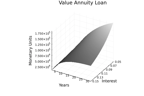
Source: own presentation.
The examples can now be extended and modified as required. The values calculated below can no longer be determined using the above formulae as a substitute and a linear or non-linear programme ( base program and valuation program) must be drawn up in accordance with functional valuation theory.
The following is a variation with 10000 MU equity from Immanuel Biele. Why do the values change? In the base case of the rent (base program), the withdrawal flow increases by the interest on equity (corrected by a growth discount if necessary).This increased withdrawal flow must also be achieved in the case of acquisition (valuation program). In the case of the acquisition (valuation program), however, it is worthwhile not to invest the money but to avoid the expensive interest repayment of 10%. In addition, the loan can be increased in volume. (In the end, more interest is paid, but there is no longer a low-interest investment.) The values below just allow the same withdrawal flow as in the base program. (The decision value is the maximum acceptable acquisition price at which the advantageousness changes.)
Table 11: Variation Acquisition with Equity
| Case | without Growth | with Growth |
|---|---|---|
| Acquisition: Maximum Acceptable Acquisition Price (Unlimited Debt) | 126250.0 | 157812.5 |
| Acquisition: Maximum Acceptable Acquisition Price (Net Present Value) | 81430.59 | 88344.30 |
Source: own presentation.
In a further variation, Immanuel Biele waives 50% of his non-compulsory consumption (withdrawal) for 10 years in the case of both renting and acquiring.
In the case of renting (base program), he can invest the money and receive interest. In particular, he saves up to year 10 and receives interest.
In the case of acquisition (valuation program), two groups of cases are presented. Firstly, he, and of course his house bank, allows unlimited debt. Alternatively, the real estate is paid off within 10 years.
Table 12: Variation Acquistion and Rent with and without Growth and 50% Waiver of Withdrawal for 10 Years
| Case | without Growth | with Growth |
|---|---|---|
| Rent: Ersparnis im Jahr 10 | 63099.85 | 76836.95 |
| Acquisition: Maximum Acceptable Acquisition Price (Unlimited Debt) | 143547.02 | 182930.16 |
| Acquisition: Maximum Acceptable Acquisition Price (Net Present Value) | 106404.72 | 118914.13 |
Source: own presentation.
As you can see, there is no “value” that is universally valid for everyone. The decision value depends on the subject of the valuation and his situation. Nevertheless, it can be simplified. The approximation is carried out using the original capitalised earnings method, which represents a simplification of the functional valuation approach and is less complicated. This is comparatively simple and now follows.
The easiest way to do the calculation is with the Julia programming language and not with Excel or an online calculator. The inhibition threshold may be a little higher, but Julia has a philosophy that you only need to understand as much as is absolutely necessary. It will remain very easy here. You don’t need any programming skills.
The calculations above were essentially carried out with a linear programme (operations research) of functional valuation theory (functional business valuation). The following calculations are carried out using the original capitalised earnings method. You can do this too!
Follow the instructions under capitalised earnings method calculator and come back here. Calculations for all examples except the “Variations” follow. You can copy the examples by right-clicking on them. However, do not copy the equals sign and the solution. The function is structured as follows:
capitalised_earnings(net cash flow, net interest, growth=0.02, risk=0.0, years=false)
The net cash flow and net interest must be entered, the rest is optional. The growth has a default value of 0.02, the risk of 0.0 and the years the value “false”. For the years, “false” means that a perpetual annuity is calculated at the end. If the years are specified, a present value is discounted at the end and not a perpetual annuity. For the consideration of risk, please refer to the corresponding section on the capitalised earnings value method.
Sale with perpetual annuity
capitalised_earnings(12000*(1-0.3), 0.05*(1-0.25)) = 224000
Sale with perpetuity and growth
capitalised_earnings(12000*(1-0.3), 0.05*(1-0.25), 0.02) = 480000
Acquisition (interest only case) with perpetuity
capitalised_earnings(12000, 0.1, 0) = 120000
Acquisition (interest only) with perpetuity and growth
capitalised_earnings(12000, 0.1, 0.02) = 150000
Acquisition (annuity loan case) with cash value
capitalised_earnings(12000, 0.1, 0.0, 0.0, 10) = 73734.81
Acquisition (annuity loan case) with cash value and growth
capitalised_earnings(12000, 0.1, 0.02, 0.0, 10) = 79503.73
Of course, it is best to set up a linear or non-linear programme (operations research). This can be used to simulate many more subtleties (e.g. progressive taxes, loss carryforwards, various alternative investments, different withdrawal preferences, etc.). Walochnik (2021) has done excellent work on the topic in relation to real estate in his PhD thesis. But I also like to use the capitalised earnings method to estimate the value of real estate and a company.
© All Rights Reserved 2023