
The discounted cash flow (DCF) method is a generic term for various approaches for calculating the company value or the real estate value (valuation object). In summary, the future cash flow is discounted to the present time and expressed as the company value.
Are you looking for a business consultant to help you with your business valuation using the DCF method? Get in touch for a free initial consultation.
The adjusted present value (APV) approach, the weighted average capital cost (WACC) approach and the total cash flow (TCF) approach belong to the entity approaches (gross methods). The flow-to-equity (FTE) approach is an equity approach (net method). The TFC approach is omitted in the following.
First, the basics of the DCF method are explained. Then three different approaches, namely the AVP approach, the WACC approach and the equity approach are presented in more detail. This is followed by a comparison between the capitalised earnings method and the DCF method.
DCF methods are based either on the equilibrium model of Modigliani and Miller (1958), or on the capital asset pricing model (Sharpe, 1964; Lintner, 1965; Mossin, 1966).
According to the equilibrium model of Modigliani and Miller (1958), investors can invest in shares and bonds of companies on a capital market. The investors’ expectations about the expected return, the risk of the companies’ profit distributions and a risk-free interest rate are identical.
The value of a company results from the discounted profit distributions and bonds. Profit distributions are discounted using the cost of equity and debt using the cost of debt.
Basically, this also assumes tax neutrality of equity and debt capital as well as a lack of bankruptcy risk.
By the way, there is a competing model with the classical thesis. In this model, the debt-equity ratio has an impact on the total cost of capital, which is not linear.
The assumptions are, among others:
It can be seen that these assumptions are not fulfilled in reality. It is a simplified explanatory model.
The capital asset pricing model is based on the portfolio theory of Markowitz (1952) and the equilibrium model of Modigliani and Miller (1958). It can be attributed to three authors (Sharpe, 1964; Lintner, 1965; Mossin, 1966).
In Markowitz’s (1952) model, investors have various risky investment opportunities and skillfully combine them so that the expected return is realised with minimal risk. In Makrowitz’s model, one speaks of an efficient frontier, which specifies the optimal combination possibilities of expected returns and risks.
The model can be extended to include a risk-free interest rate for investing or borrowing money. One then has a so-called tangential portfolio. In summary, an attempt is made to achieve an expected return with the lowest possible risk (variance) by cleverly combining investments.
The CAPM model now assumes that all investors have the same expectations about the returns on the capital market. Investors can invest money in assets and invest or borrow money on the financial market accordingly. Through an “invisible hand”, the market values and thus the company values are determined for the market equilibrium. The result is a so-called market portfolio with a capital market line.
The expected return is determined by a price of time (risk-free interest rate) and price of risk (risk premium). For the mathematical derivation, please refer to the sources mentioned. They will probably be familiar to some readers. The systematic risk can be expressed as market risk premium * beta factor.
The formula for the capital market line in the CAPM model is:
expected return = risk-free rate + (expected return market portfolio – risk-free rate)/ standard deviation market portfolio * standard deviation
For the individual investor, the expected value depends upon the portfolio risk taken (standard deviation). More information on this can be found in the cited literature.
The formula for the security line in the CAPM model is:
expected return = risk-free interest rate + (expected return on market portfolio- risk-free interest rate)/standard deviation market portfolio^2 * covariance of the investment relative to the market portfolio
However, the formula of the security line in the CAPM model is often presented as follows:
expected return = risk-free interest rate + (market risk-risk-free interest rate) * beta factor
The assumptions of the model are, among others:
When considering the assumptions, it also becomes clear that this is a simplified explanatory model and does not reflect reality. While some assumptions are removed by model extensions, such as in Brennan (1970) for tax integration, the basic critique remains.
The risk measurement based on variance also causes positive desired deviations to lead to greater discounting, which does not seem reasonable from the theoretical side.
It should be noted that the equilibrium model of Modigliani-Miller and CAPM are actually not combinable from the risk propensity and time horizon (Hering, 2021).
The gross profit of a company is 12000 (MU). The tax rate is 30%. The company has borrowed capital worth (1000/0.05) = 20000 MU. The interest rate in each period is 5% and the interest expense is 1000 MU. Interest is tax deductible.
Gross profit is 12000 MU and after tax (30%) 12000-(12000-1000)*0.3 = 8700 MU is distributed to the owners (net cash flow).
However, without the benefit of debt, the net profit would only be 10000-(12000)*0.3 = 8400 MU (equity-financed net cash flow).
In the following explanations, an equivalence of the three DCF approaches is established so that the connection is easy to understand. In addition, a perpetual annuity is used first for easier understanding, so that problems such as the optimal capital structure can be ignored.
For a similar example with a piecewise inductive explanation, please refer to the example of the capitalised earnings method, for this moment only available in German.
Discounted cash flow means that the cash flow is discounted. The basic formulas for this will be presented here. In the case of a perpetual annuity, the net present value results from the following formula:
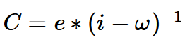
C stands for the net present value, e for the cash flow, i for the interest rate and ω for the growth rate. For example, a perpetual cash flow of 12000 MU, with an interest rate of 5% and a perpetual growth rate gives 12000/(0.05-0.02)= 400000 MU.
For period-specific discounting, the discount factor ρ must be calculated for each period in order to be able to discount the cash flow later. In the following formula, t stands for the year and τ is a running variable.
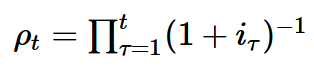
For example, with two periods and an interest rate of 5%, discount factors result in 1.05^-1*1.05^-1=0.90702 and 1.05^-1=0.9524.
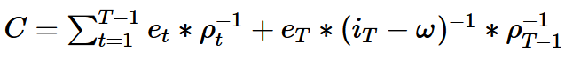
When divided into a detailed planning period and a residual value, the total company value can be determined as follows. First, the cash flow within the planning period is discounted. Then a perpetual annuity is applied on the planning horizon, which is also discounted again with a discount factor.
In the following formula, T stands for the planning horizon. The remaining symbols have already been described.
The practical calculation is most easily done with the programming language Julia and not with Excel or an online calculator. The inhibition threshold may be a little higher, but Julia has a philosophy that only as much as is absolutely necessary needs to be understood. Here it will remain very easy. You don’t need any programming knowledge.
Download Julia here and install it.
Start Julia by clicking on the icon on the desktop, or in the menu.
Copy the following code and paste it into Julia (REPL) with a right click. Then press Enter and the important function for discounting npv (net present value) is saved in the session. The function is important for the approaches still to be described.
terminalvalue(val,i,g,n) = val*(1-(1+g)^n*(1+i)^-n)/(i-g)
terminalvalue(val,i,g,n::Bool) = val/(i-g)
function npv(interest, cashflow, growth=0.02,n=false)
cashflow = copy(cashflow)
@assert length(interest) == length(cashflow)
if length(cashflow) == 1
terminalvalue(cashflow[1],interest[1],growth[1],n)
else
discount_factor = cumprod([(1+i)^-1 for i in interest])
cashflow[end] =
terminalvalue(cashflow[end], interest[end], growth, n)
sum(cashflow[begin:end-1].*discount_factor[begin:end-1]) +
cashflow[end] * discount_factor[end-1]
end
end
# To use the examples, remove the #.
# npv(0.05,12000,0.02) # Example for perpetuity
# npv([0.05,0.05,0.05], [12000,12240,12484.8], 0.02) # Example of a detailed planning period with subsequent perpetuity
# npv([0.05,0.05,0.05], [12000,12240,12484.8], 0.02, 10) # Example of a detailed planning period with subsequent present value
The adjusted present value (APV) approach is a variant of the DCF method and is based on the equilibrium model of Modigliani and Miller (1958) and can be traced back to Myers (1974).
The company value results from a basic present value of the debt-free company plus a tax shield. The tax shield arises because debt capital is tax privileged. If the value of the debt is subtracted from the total company value, the cost of equity can be calculated in retrospect. These can also be used to create an equivalence to the WACC approach and the equity approach.
First, the company value is calculated as a perpetual annuity without growth (steady state). In the case of a steady state, there is a smooth equivalence between the APV approach, WACC and equity approach.
The owner expects a return of 10%.
For the APV approach, the self-financed free cash flow of 8400 MU is used to calculate the basic net present value. This is discounted by the expected return of 10% (8400 / 0.1 = 84000 MU).
The tax shield results from the net value of the debt, which was already calculated above as 20000 MU, by multiplying this by the tax rate of 30%. The result is 20000 * 0.3 = 6000 MU.
The basic net present value and the net present value of the tax shield together result in the company value including debts of 84000 + 6000 = 90000 MU.
If the net present value of the debt is subtracted, the value of the equity (“company value”) is 90000 – 20000 = 70000 MU.
From this the equity costs of 0.1+(1-0.3)*(0.1-0.05)*(20000/70000) = 11% can be derived. Alternatively, the following calculation method is also possible (8700-1000)/70000 = 11%.
The approach is now to be extended so that the first two years represent a detailed planning period and then a perpetual annuity with a perpetual growth rate is applied. The procedure is identical to the above example, except that discounting is first carried out on a period-specific basis and then with the help of a perpetual annuity including a growth rate. The formula described above is used.
The basic cash value is npv([0.1,0.1,0.1], [8400.0, 8568.0, 8739.36], 0.02) = 105000 MU.
The present value of the debt is npv([0.05,0.05,0.05], [1000.0, 1020.0, 1040.4] , 0.02) = 33333.34 MU.
The present value of the tax shield is npv([0.05,0.05,0.05], [1000.0, 1020.0, 1040.4] .* [0.3, 0.3, 0.3] , 0.02) = 10000 MU.
The value of the company including debts is 105000 + 10000 = 115000 MU.
The value of the equity (company value) is 115000 – 33333.34 = 81666.67 MU.
The cost of capital must be calculated iteratively per period. In the first period it is
0.1+(1-0.3)*(0.1-0.05)*(33333.34/81666.67) = 0.1142857142857143.
The data here was chosen so that the cost of capital remains the same in the following periods.
function apv_internal(i_equity,i_debt, taxrate, net_profit, i_expenses, growth,period)
base_npv = npv(i_equity, net_profit, growth)
debt_npv = npv(i_debt, i_expenses, growth)
tax_shield_npv = npv(i_debt, i_expenses .* taxrate, growth)
company_value = base_npv + tax_shield_npv
equity_value = company_value – debt_npv
i_apv = i_equity[1] +(1 – taxrate[1])*
(i_equity[1]-i_debt[1])*(debt_npv/equity_value)
printstyled(“Data for the $period. period:\n”,bold=true,color=:cyan)
for (text, val) in
zip([“equity:”,”debt:”,”total value:”,”tax shild:”,”i_apv:”],
[equity_value,debt_npv,company_value,tax_shield_npv,i_apv])
println(rpad(text,15),round(val,digits=4))
end
nothing
function apv(i_equity,i_debt, taxrate, net_profit, i_expenses, growth)
period = length(net_profit)
for i in 1:period
apv_internal(i_equity[i:end],i_debt[i:end], taxrate[i:end],
net_profit[i:end], i_expenses[i:end],growth,i)
end
end
# To use the example, remove the # character below.
# apv([0.1,0.1,0.1],[0.05,0.05,0.05],[0.3,0.3,0.3],[8400.0, 8568.0, 8739.36], [1000.0, 1020.0, 1040.4],0.02)
The weighted average cost of capital (WACC) approach is a variant of the DCF method and is based on the CAPM model (Sharpe, 1964; Lintner, 1965; Mossin, 1966).
In addition to the initial data, the equity capital costs are taken from the APV approach of 11%. Equivalence to the APV approach can be achieved without any difficulties. The formula for WACC is:
WACC = cost of equity * value of equity / value of total capital + (1 – tax) * cost of debt * value of debt / value of total capital
WACC = 0.11*(70000/90000)+(1-0.3)*0.05*(20000/90000) = 9,33%
If the equity-financed free cash flow of 8400 MU is discounted with WACC, the result is 8400/0.0933 = 90000 MU.
From the total company value of 9000 MU, the debts of 20000 MU must again be subtracted, so that the equity is worth 70000 MU.
In practice, WACC is not seen as a reformulation of the APV approach, but the cost of equity is derived from the CAPM model.
If an equivalence to the APV approach is attempted in the case with a detailed planning period and a perpetuity with growth rate, the results may be unsatisfactory. Specifically, for equivalence between the APV approach and WACC, a distinction must be made between the present value of the tax shield and the value of the latter. The net present value is determined with the interest rate on borrowed capital. The value is first discounted using the borrowing rate (existing debt) and then using the cost of equity (new debt). For a derivation and reconciliation, please refer to Massari et al. (2008).
In practice, the cost of equity for WACC is not calculated as a reformulation of the APV approach, but is derived from the CAPM model. At the end of the period, the perpetuity with growth corresponding to equity-financed cash flow/(WACC – growth rate) is applied and discounted with a discount factor. It may be that many practical users are not really aware of the problem and “simply” apply the formulas.
The flow-to-equity (FTE) approach is a variant of the DCF method and is based on the CAPM model (Sharpe, 1964; Lintner, 1965; Mossin, 1966).
The free cash flow is discounted using the cost of equity. However, the interest on debt must be subtracted from the net cash flow (incl. tax advantage). If the data from the APV approach is used, this would be (8700-1000)/0.11 = 70000 MU.
Equivalence can be established between the equity approach and the APV approach.
In practice, the cost of equity is not derived from the APV approach, but from the model CAPM.
The interest rate is again taken from the APV approach. The result of the equity approach and the APV approach match.
npv([0.1142857142857143,0.1142857142857143,0.1142857142857143], [8700.0, 8874.0, 9051.48] – [1000.0, 1020.0, 1040.4],0.02) = 81666.67 MU
In the following, the capitalised earnings method will be compared to the DCF method and an example will be given for both.
The data are from the given scenario with growth rate. Inflation and thus cash flow increase of 2% are assumed, which results in a perpetual growth rate at the planning horizon. The interest rate is 5% but must be taxed at 25% on private assets, so the net interest rate is 3.75%. There is no tax on the profit from the sale of the company.
The seller subjectively sees the expectations about the company’s development as certain. Furthermore, he is risk averse and wants to invest the proceeds from the sale of the company at the bank.
According to the (original) capitalised earnings method, the company value is 8700/(0.0375-0.02) = 497142.86 MU. In order to get the same net cash flow as from the company shares, the seller must invest an amount of 497142.86 MU at the bank.
If the interest rate or the cash flow fluctuates within the planning period, the more complicated formula with period-specific discounting factors must be applied. As an example, it is applied here to the case of perpetuity with growth rate:
Year 1: 8700 * (1+0.0375)^-1 = 8385.54 MU
Year 2: 8874 * (1+0.0375)^-1 * (1+0.0375)^-1 = 8.244,1 MU
Year 3: 9051.48/(0.0375-0.02) * (1+0.0375)^-1 * (1+0.0375)^-1 = 480513,22 MU
The sum is exactly 497142.86 MU.
Capitalised Earnings Method Example
| Name | Year 1 | Year 2 | Year 3 | Year... |
|---|---|---|---|---|
| capital | 497142.86 | 505842.86 | 514673.36 | ... |
| interest revenue (gross) | 24857.14 | 25292.14 | 25733.67 | ... |
| taxes | -6214.29 | -6323.04 | -6433.42 | ... |
| withdrawal | -8700 | -8874 | -9051.48 | ... |
Source: own representation.
The calculations show that every year he receives the same cash flow as through his former company. Since the cash flow grows forever, the invested capital also increases in each period.
The company value is now calculated using the equity approach, which is equivalent to the APV approach from above. The data are taken from the above example of the APV approach and the equity approach with a perpetual growth rate of 2% in the steady state.
(8700-1000)/(0.1142857142857143-0.02) = 81666.67 MU.
If the interest rate or the cash flow fluctuates within the planning period, the more complicated formula with period-specific discounting factors must also be applied here. As an example, it is applied here to the case of a perpetual annuity with a growth rate:
Year 1: (8700-1000)* (1+0.1142857142857143)^-1 = 6910.26 MU
Year 2: (8874-1020)* (1+0.1142857142857143)^-1 * (1+0.1142857142857143)^-1 = 6325.54 MU
Year 3: (9051.48-1040.4)/(0.1142857142857143-0.02) * (1+0.1142857142857143)^-1 * (1+0.1142857142857143)^-1 = 68430.87 MU
The sum equals 81666.67 MU.
The seller sold his company for this amount because he relied on an external advisor. However, he does not invest his money on the capital market, but with his house bank at 5% gross, because he is risk averse. He tries to get the same cash flow as through the company. However, he is not able to do so and his capital decreases year by year. The problem is that the calculation was not made with the endogenous marginal interest rate of the person in question. A value was calculated for a hypothetical investor on the capital markets. The external advisor simply fell back on the textbook formulas he was familiar with, without taking the individual situation of his client into account.
DCF Method Example
| Name | Year 1 | Year 2 | Year 3 | Year... |
|---|---|---|---|---|
| capital | 81666.67 | 76029.17 | 70006.26 | ... |
| interest revenue gross | 4083.33 | 3801.46 | 3500.31 | ... |
| taxes | -1020.83 | -950.36 | -875.08 | ... |
| withdrawl | -8700 | -8874 | -9051.48 | ... |
Source: own representation.
The DCF method is based on theoretical models of the capital market, which do not correspond to the real world. In the above example, the alternative investment was the interest rate given by the bank (endogenous marginal interest rate) and not an interest rate derived from the CAPM model. The extreme example shows that the decision value of the subject only coincidentally corresponds to the company value, which is calculated using the DCF method.
The divergence of the company value according to the DCF method can occur both upwards and downwards in comparison to the capitalised earnings method or functional business valuation.
The different approaches of the DCF method are based on the equilibrium model of Modigliani and Miller (1958) or the CAPM model of (Sharpe, 1964; Lintner, 1965; Mossin, 1966). The premises for these explanatory models are not given in real imperfect markets. However, the assumptions of the second model are more restrictive than those of the first model.
What is generally problematic about DCF methods is that they do not take into account the individual situation of the investor with his real investment opportunities, his tax rates and his withdrawal preferences. A fictive company value is calculated for a fictive investor who operates on perfect capital markets. However, this value will only very rarely match the decision value of the actual investor. To calculate this, we must apply the functional business valuation or the closely related capitalised earnings method. Only this method allows the integration of these subtleties into a valuation model. For a detailed critique, please refer to Hering (2017), Hering (2021) and Matschke and Brösel (2013).
In practice, the decision value, which marks the cut-off point for advantageousness, should be determined according to the functional business valuation. In addition, argumentation values can be calculated on the basis of different DCF approaches and other methods for business valuation. This provides an excellent information basis with a respective negotiating position.
Hering, T. (2017). Investitionstheorie (5th ed.). De Gruyter Oldenbourg.
Hering, T. (2021). Unternehmensbewertung (5th ed.). De Gruyter Oldenbourg.
Markowitz, H. (1952). Portfolio Selection. The Journal of Finance, 7(1), 77-91.
Terstege, U, Bitz, M. & Ewert, J (2023). Investitionsrechnung klipp & klar. Springer Gabler.
© All Rights Reserved 2023